Stanford CS336: lecture 2 Pytorch, Resource Accounting

主要介绍训练模型所需的基本要素，从张量到模型、再到优化器与训练循环，强调资源效率，尤其是内存（GB）与计算量（FLOPs）的核算。课程不涉及 Transformer，而是通过更简单的模型来讲解。

学习目标包括：

机制：掌握基本的 PyTorch 用法；
思维方式：学会资源核算；
直觉：把握整体理解，而非大规模模型细节。

主要内容：

内存核算：张量基础与内存管理
计算核算：GPU 上的张量操作、Einops、操作 FLOPs、梯度计算与 FLOPs
模型：参数模块与自定义模型
训练循环与实践：随机性说明、数据加载、优化器、训练循环、检查点保存、混合精度训练

动机问题与“纸上估算”摘要：

目标：用粗略估算评估训练时间与可训练的最大模型规模。
问题1（训练时间）：训练 700 亿参数模型、15T tokens、1024 张 H100。
- 假设：h100_flop_per_sec = 1979e12 / 2，mfu = 0.5。
- 公式：
  - total_flops = 6 * 70e9 * 15e12
  - flops_per_day = h100_flop_per_sec * mfu * 1024 * 60 * 60 * 24
  - days = total_flops / flops_per_day
问题2（最大模型规模）：在 8 张 H100 上用 AdamW（朴素实现）能训练的最大参数量。
- 假设：每卡显存 h100_bytes = 80e9；每参数内存：4（参数）+4（梯度）+(4+4（优化器状态）)=16 字节。
- 公式：num_parameters = (h100_bytes * 8) / 16。
注意事项：
1. 朴素地用 float32 表示参数与梯度；也可用 bf16（2+2）并保留一份 fp32 参数副本（4），速度更快但不省显存。
2. 未计入激活开销（依赖 batch size 与序列长度）。
  
  以上为粗略估算。

张量

张量基础

张量是存储一切内容的基本构件，包括参数、梯度、优化器状态、数据与激活。

在 PyTorch 中可通过多种方式创建张量：

torch.tensor([[1., 2, 3], [4, 5, 6]])：直接定义二维张量
torch.zeros(4, 8)：4×8 全零矩阵
torch.ones(4, 8)：4×8 全一矩阵
torch.randn(4, 8)：4×8 标准正态分布随机矩阵
torch.empty(4, 8)：4×8 未初始化矩阵（可自定义填充值）

未初始化张量常用于后续用特定逻辑赋值，例如：

nn.init.trunc_normal_(x, mean=0, std=1, a=-2, b=2) 进行截断正态初始化。

张量内存

存储内容：几乎所有数据（参数、梯度、激活、优化器状态）都以浮点数形式存储。
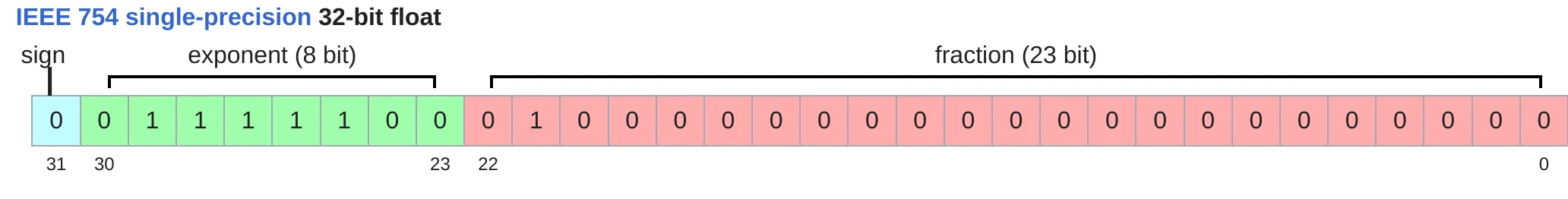
float32（fp32，单精度）
- 默认数据类型，每个数占 4 字节。
- 示例：torch.zeros(4,8) → 占用 4*8*4=128 字节。
- GPT-3 前馈层中的一个大矩阵可达 2.3 GB。
float16（fp16，半精度）
- 每个数 2 字节，节省内存。
- 动态范围有限，容易下溢：如 1e-8 → 0。训练中可能导致不稳定。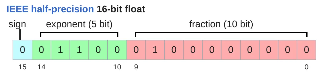
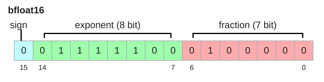
bfloat16（bf16）
- Google Brain 2018 提出。
- 占用与 float16 相同内存，但动态范围与 float32 相同，仅分辨率较差。
- 解决了 float16 下溢问题，更适合深度学习。
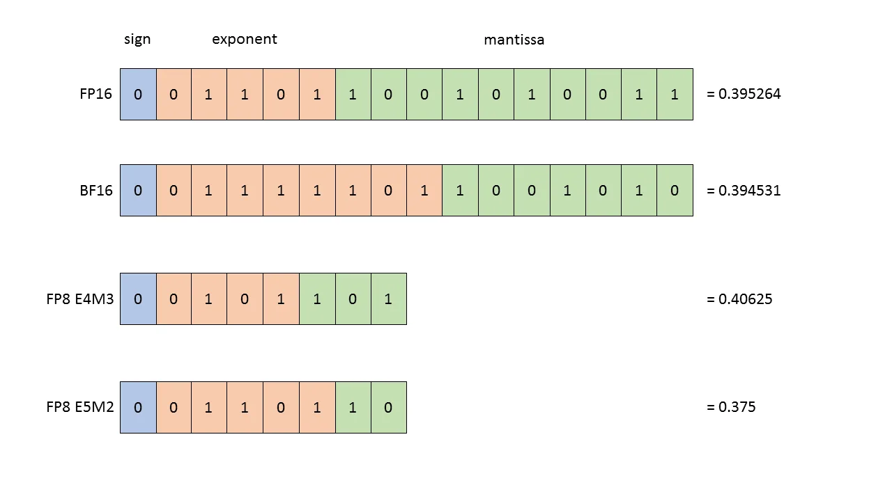
fp8
- 2022 年标准化，专为机器学习设计。https://docs.nvidia.com/deeplearning/transformer-engine/user-guide/examples/fp8_primer.html
- H100 支持两种：E4M3（范围 -448448）、E5M2（范围 -5734457344）。 [Micikevicius+ 2022]
训练影响：
- float32 稳定但耗内存。
- fp8、float16、bfloat16 内存更省，但可能带来数值不稳定。
- 解决方案：采用混合精度训练（后续介绍）。

张量在GPU上使用

默认情况：张量存储在 CPU 内存中，如 torch.zeros(32, 32) → 设备为 cpu。

content-image-1

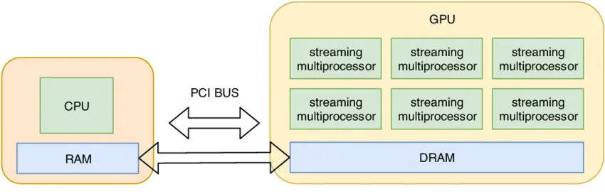
利用 GPU 并行性：需将张量转移到 GPU 内存。
- 检查 GPU 可用性：torch.cuda.is_available()
- 获取 GPU 数量：torch.cuda.device_count()
- 查看设备属性：torch.cuda.get_device_properties(i)
- 查看已分配内存：torch.cuda.memory_allocated()
将张量转移到 GPU：
- y = x.to("cuda:0") → 张量移至 0 号 GPU。
直接在 GPU 创建张量：
- z = torch.zeros(32, 32, device="cuda:0")
- GPU 内存消耗变化：memory_used = 2 * (32 * 32 * 4) → 8192 字节。

张量操作

总体：大多数张量来源于对已有张量的操作，每个操作都有内存与计算代价。

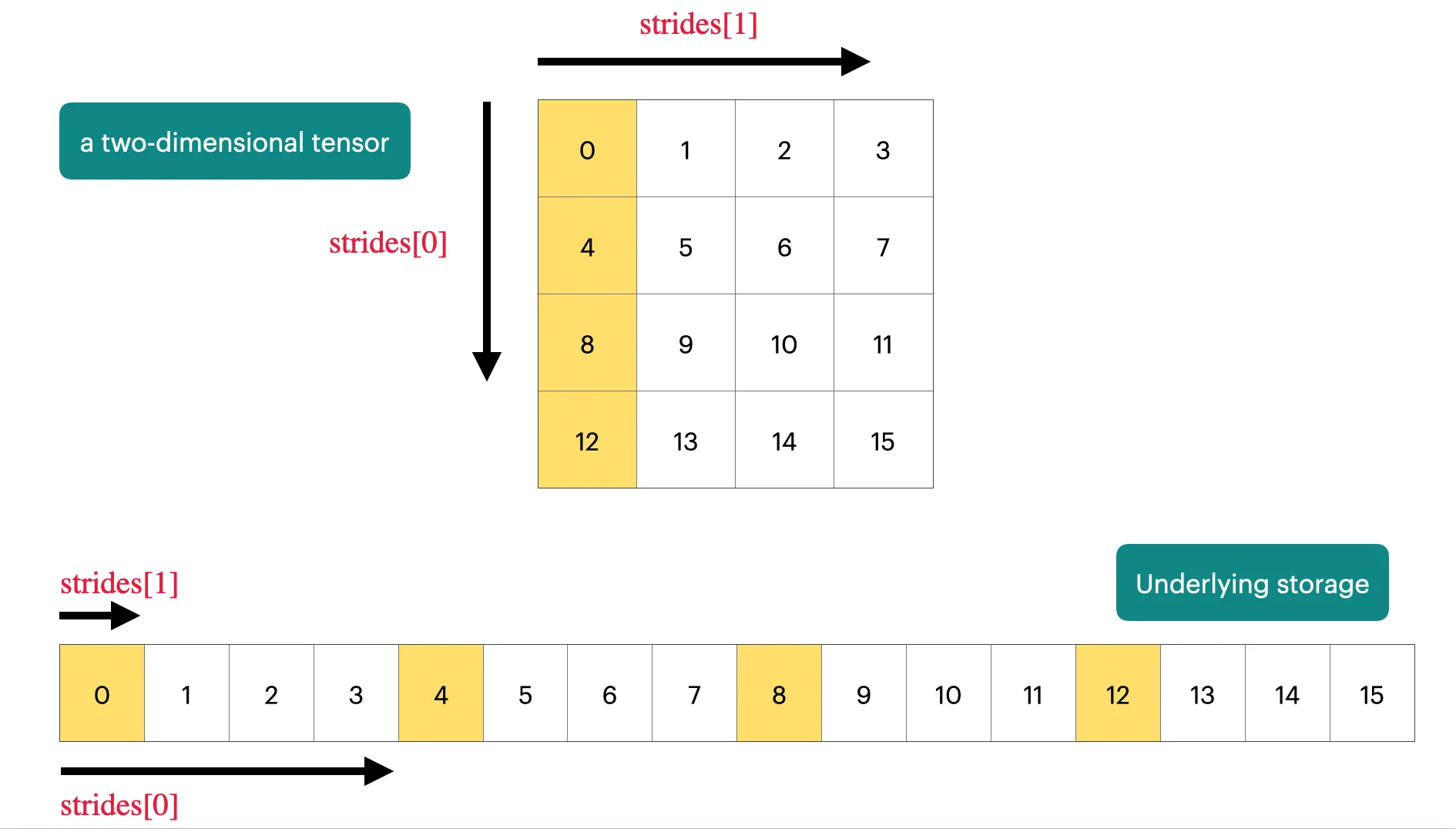
1. 存储（tensor_storage）[PyTorch docs]

张量本质是指向已分配内存的指针，加上元数据描述。
访问元素通过 stride（步长） 定位，例如行步长为 4，列步长为 1。
示例：x[1,2] 对应存储索引 1*4 + 2*1 = 6。

content-image-1

python

import torch

# 创建一个 4x4 张量
x = torch.tensor([
    [0., 1, 2, 3],
    [4, 5, 6, 7],
    [8, 9, 10, 11],
    [12, 13, 14, 15],
])

# 张量的 stride 表示在某一维度上移动一个单位所需跳过的元素数
# dim=0 表示行方向，每下一行需要跳过 4 个元素
assert x.stride(0) == 4

# dim=1 表示列方向，每下一列需要跳过 1 个元素
assert x.stride(1) == 1

# 查找某个元素在内存中的索引
r, c = 1, 2
index = r * x.stride(0) + c * x.stride(1)  # 行偏移 + 列偏移
assert index == 6

print("张量：\n", x)
print("stride:", x.stride())
print(f"元素 x[{r}, {c}] 在存储中的索引: {index}, 值为: {x[r, c].item()}")

2. 切片与视图（tensor_slicing）

切片操作（取行、取列、转置、reshape 等）通常返回视图，不复制数据，修改原张量会影响视图。
若视图是非连续内存（如转置），某些操作（如 .view()）会报错，需要先 .contiguous()。
视图开销为 0，复制操作则额外消耗内存和计算。

python

import torch

def same_storage(a: torch.Tensor, b: torch.Tensor) -> bool:
    """判断两个张量是否共享底层存储"""
    return a.storage().data_ptr() == b.storage().data_ptr()

# =========================================
# 张量视图 (View) 基础
# =========================================
x = torch.tensor([[1., 2, 3], [4, 5, 6]])  # @inspect x

# 1. 获取第 0 行
y = x[0]  # @inspect y
assert torch.equal(y, torch.tensor([1., 2, 3]))
assert same_storage(x, y)   # 共享存储

# 2. 获取第 1 列
y = x[:, 1]  # @inspect y
assert torch.equal(y, torch.tensor([2, 5]))
assert same_storage(x, y)   # 共享存储

# 3. 将 2x3 矩阵重新视为 3x2 矩阵
y = x.view(3, 2)  # @inspect y
assert torch.equal(y, torch.tensor([[1, 2], [3, 4], [5, 6]]))
assert same_storage(x, y)

# 4. 转置矩阵
y = x.transpose(1, 0)  # @inspect y
assert torch.equal(y, torch.tensor([[1, 4], [2, 5], [3, 6]]))
assert same_storage(x, y)

# 5. 修改原张量，视图也会同步改变
x[0][0] = 100  # @inspect x, @inspect y
assert y[0][0] == 100

# =========================================
# 非连续存储 (Non-contiguous) 的限制
# =========================================
x = torch.tensor([[1., 2, 3], [4, 5, 6]])  # @inspect x
y = x.transpose(1, 0)  # @inspect y
assert not y.is_contiguous()

# 尝试对非连续张量直接 view 会报错
try:
    y.view(2, 3)
    assert False
except RuntimeError as e:
    assert "view size is not compatible with input tensor's size and stride" in str(e)

# 解决方法：先 contiguous() 再 view
y = x.transpose(1, 0).contiguous().view(2, 3)  # @inspect y
assert not same_storage(x, y)  # 复制了存储

3. 元素级操作（tensor_elementwise）

对张量逐元素计算，返回相同形状的新张量。
示例：pow、sqrt、+、、/ 等。
triu 可取上三角矩阵，常用于因果注意力掩码。

python

import torch

# =========================================
# 张量的逐元素操作 (Element-wise operations)
# =========================================
x = torch.tensor([1, 4, 9])

# 幂运算
assert import torch

# =========================================
# 张量的逐元素操作 (Element-wise operations)
# =========================================
x = torch.tensor([1, 4, 9])   # 每个元素平方

# 开方
assert torch.equal(x.sqrt(), torch.tensor([1, 2, 3]))     # 每个元素开方

# 取倒数开方 (1/sqrt)
assert torch.equal(x.rsqrt(), torch.tensor([1, 1/2, 1/3]))

# 加法
assert torch.equal(x + x, torch.tensor([2, 8, 18]))

# 乘法
assert torch.equal(x * 2, torch.tensor([2, 8, 18]))

# 除法
assert torch.equal(x / 0.5, torch.tensor([2, 8, 18]))

# =========================================
# 上三角矩阵 (Upper triangular matrix)
# =========================================
x = torch.ones(3, 3).triu()  # @inspect x

expected = torch.tensor([
    [1, 1, 1],
    [0, 1, 1],
    [0, 0, 1],
])
assert torch.equal(x, expected)

# 这种上三角掩码常用于 **因果注意力 (causal attention mask)**，
# 其中 M[i, j] 表示位置 i 对位置 j 的贡献是否允许。

4. 矩阵乘法（tensor_matmul）

深度学习的核心操作。
示例：(16,32) @ (32,2) → (16,2)。
批量与序列维度会自动广播迭代，如 (4,8,16,32) @ (32,2) → (4,8,16,2)。

content-image-1

python

import torch

# =========================================
# 深度学习核心操作：矩阵乘法 (Matrix Multiplication)
# =========================================

# 单个矩阵乘法示例
x = torch.ones(16, 32)  # 输入矩阵：16 行 32 列
w = torch.ones(32, 2)   # 权重矩阵：32 行 2 列

y = x @ w  # 矩阵乘法
assert y.size() == torch.Size([16, 2])
print("y.shape:", y.shape)  # 输出: torch.Size([16, 2])

# =========================================
# 批处理和多维矩阵乘法
# =========================================
# 假设有一个 4 维张量，表示 batch x seq_len x dim1 x dim2
x = torch.ones(4, 8, 16, 32)
w = torch.ones(32, 2)

# 对最后两个维度执行矩阵乘法，前两个维度自动广播
y = x @ w
assert y.size() == torch.Size([4, 8, 16, 2])
print("y.shape (batch & sequence):", y.shape)

# 说明：
# 对于多维张量，矩阵乘法会在前面多余的维度上迭代，
# 类似于对每个 batch 和序列位置分别进行乘法。

Einops张量操作

Einops 是一个用于操作张量的库，其中的维数都是命名的。它的灵感来自爱因斯坦求和符号（爱因斯坦，1916 年）。[Einops tutorial]

Einops 动机：

提供以命名维度操作张量的方法，避免传统 PyTorch 操作中维度易混乱的问题（如 2, -1）。

python

import torch

# =========================================
# 批次与序列维度的矩阵乘法 (Batch & Sequence Matrix Multiplication)
# =========================================

# 输入张量：batch x sequence x hidden
x = torch.ones(2, 2, 3)  # @inspect x
y = torch.ones(2, 2, 3)  # @inspect y

# 对最后两个维度做矩阵乘法
# 注意 y 需要转置最后两个维度 (-2, -1) 才能匹配 x 的最后一维
z = x @ y.transpose(-2, -1)  # 结果 shape: batch x sequence x sequence  @inspect z

print("x.shape:", x.shape)  # torch.Size([2, 2, 3])
print("y.shape:", y.shape)  # torch.Size([2, 2, 3])
print("z.shape:", z.shape)  # torch.Size([2, 2, 2])

jaxtyping

为张量维度加注释，便于文档化维度信息，例如：

x: Float[torch.Tensor, "batch seq heads hidden"]

python

import torch
from jaxtyping import Float

# =========================================
# 张量维度管理示例 (Tracking Tensor Dimensions)
# =========================================

# 传统方式 (Old way)
x = torch.ones(2, 2, 1, 3)  # batch, seq, heads, hidden  @inspect x
print("x.shape (old way):", x.shape)  # torch.Size([2, 2, 1, 3])

# 新方式 (jaxtyping 风格，主要用于文档注释)
x: Float[torch.Tensor, "batch seq heads hidden"] = torch.ones(2, 2, 1, 3)  # @inspect x
print("x.shape (jaxtyping):", x.shape)  # torch.Size([2, 2, 1, 3])

# 注意：
# - jaxtyping 的注释只是文档说明，并不会强制类型或 shape。
# - 对大型模型或复杂张量计算，使用这种注释可以更清楚地记录维度语义。

einsum（推广矩阵乘法）：

通过命名维度进行张量乘法，未在输出中出现的维度会被求和。
支持 ... 表示任意数量维度的广播。

python

import torch
from jaxtyping import Float
from torch import einsum

# =========================================
# 通用矩阵乘法：Einsum 示例
# =========================================

# 定义张量，使用 jaxtyping 注释维度
x: Float[torch.Tensor, "batch seq1 hidden"] = torch.ones(2, 3, 4)  # @inspect x
y: Float[torch.Tensor, "batch seq2 hidden"] = torch.ones(2, 3, 4)  # @inspect y

# -----------------------------------------
# 传统方式：矩阵乘法 + 转置
# -----------------------------------------
# 计算序列间相似度矩阵
z = x @ y.transpose(-2, -1)  # shape: batch x seq1 x seq2  @inspect z
print("z.shape (traditional):", z.shape)  # torch.Size([2, 3, 3])

# -----------------------------------------
# 新方式：einsum（使用命名维度）
# -----------------------------------------
# 明确维度对应关系
z_einsum = einsum("b i h, b j h -> b i j", x, y)
print("z_einsum.shape:", z_einsum.shape)  # torch.Size([2, 3, 3])

# 使用 ... 表示任意数量的前置维度（广播）
z = einsum("b i h, b j h -> b i j", x, y)
print("z.shape (torch.einsum):", z.shape)  # torch.Size([2, 3, 3])

# 说明：
# - einsum 可以自动对未在输出中出现的维度求和。
# - ... 可用于批次或额外维度的广播，简化多维计算。

reduce（降维操作）：

可对张量沿指定维度进行 sum、mean、max、min 等操作。
示例：reduce(x, "... hidden -> ...", "sum")

python

import torch
from jaxtyping import Float
from einops import reduce

# =========================================
# 张量归约操作 (Reduction)
# =========================================

# 定义张量并注释维度
x: Float[torch.Tensor, "batch seq hidden"] = torch.ones(2, 3, 4)  # @inspect x
print("x.shape:", x.shape)  # torch.Size([2, 3, 4])

# -----------------------------------------
# 传统方式：沿最后一维求均值
# -----------------------------------------
y = x.mean(dim=-1)  # @inspect y
print("y.shape (mean along hidden):", y.shape)  # torch.Size([2, 3])

# -----------------------------------------
# 新方式：einops reduce
# -----------------------------------------
# 对最后一维 hidden 进行求和
y = reduce(x, "... hidden -> ...", "sum")  # @inspect y
print("y.shape (einops sum):", y.shape)  # torch.Size([2, 3])

# 说明：
# - reduce 可以指定任意维度进行归约操作，如 "sum", "mean", "max", "min"。
# - 使用 "..." 可方便表示任意数量的前置维度，简化多维张量操作。

rearrange（重排维度）：

可将单个维度拆分为多个维度，或将多个维度合并。
示例：
- 拆分：rearrange(x, "... (heads hidden1) -> ... heads hidden1", heads=2)
- 合并：rearrange(x, "... heads hidden2 -> ... (heads hidden2)")
可与 einsum 结合进行复杂变换。

python

import torch
from jaxtyping import Float
from einops import rearrange, einsum

# =========================================
# 拆分和重组维度 + einsum 操作
# =========================================

# 定义张量，total_hidden 表示 heads * hidden1 的展开维度
x: Float[torch.Tensor, "batch seq total_hidden"] = torch.ones(2, 3, 8)  # @inspect x
print("x.shape (original):", x.shape)  # torch.Size([2, 3, 8])

# 权重矩阵
w: Float[torch.Tensor, "hidden1 hidden2"] = torch.ones(4, 4)

# -----------------------------------------
# 1. 拆分 total_hidden 为 heads 和 hidden1
# -----------------------------------------
x = rearrange(x, "... (heads hidden1) -> ... heads hidden1", heads=2)  # @inspect x
print("x.shape (after split):", x.shape)  # torch.Size([2, 3, 2, 4])

# -----------------------------------------
# 2. 对 hidden1 维度进行线性变换
# -----------------------------------------
x = einsum(x, w, "... hidden1, hidden1 hidden2 -> ... hidden2")  # @inspect x
print("x.shape (after einsum):", x.shape)  # torch.Size([2, 3, 2, 4])

# -----------------------------------------
# 3. 合并 heads 和 hidden2 回 total_hidden
# -----------------------------------------
x = rearrange(x, "... heads hidden2 -> ... (heads hidden2)")  # @inspect x
print("x.shape (after combine):", x.shape)  # torch.Size([2, 3, 8])

# 说明：
# - 这种操作常用于多头注意力或类似结构，将 flattened hidden 维度拆开处理后再合并。
# - einsum + rearrange 可以清晰地处理复杂的多维变换。

tensor_operations_flops

经过对各种张量操作的分析，需要关注它们的计算成本。浮点运算（FLOP）是基本操作，如加法或乘法。存在两个容易混淆的缩写：FLOPs 表示浮点运算的总量，用于衡量完成的计算量；FLOP/s（或 FLOPS）表示每秒浮点运算次数，用于衡量硬件的计算速度。

直觉

训练规模：
- GPT-3（2020）：约 3.14×10²³ FLOPs [article]
- GPT-4（2023）：约 2×10²⁵ FLOPs [article]
- 美国曾规定训练 ≥10²⁶ FLOPs 的基础模型需上报（2025 废止）
GPU 性能：
- A100 峰值 312 TFLOP/s [spec]
  
  a100_flop_per_sec == 312e12
- H100 峰值 1979 TFLOP/s（稀疏模式 100%，非稀疏 50%） [spec]
  
  h100_flop_per_sec == 1979e12 / 2
示例估算：
- 8 张 H100，连续运行 2 周
- 总计算量：total_flops = 8 * 60*60*24*7 * h100_flop_per_sec

线性模型

输入：n个点，每个点是d维向量。
输出：将每个d维向量映射为k个输出。

计算示例

输入点数（B）：16384
输入维度（D）：32768
输出维度（K）：8192
计算：矩阵乘法 y = x @ w。
- x 的维度为 (B, D)。
- w 的维度为 (D, K)。
- 输出 y 的维度为 (B, K)。
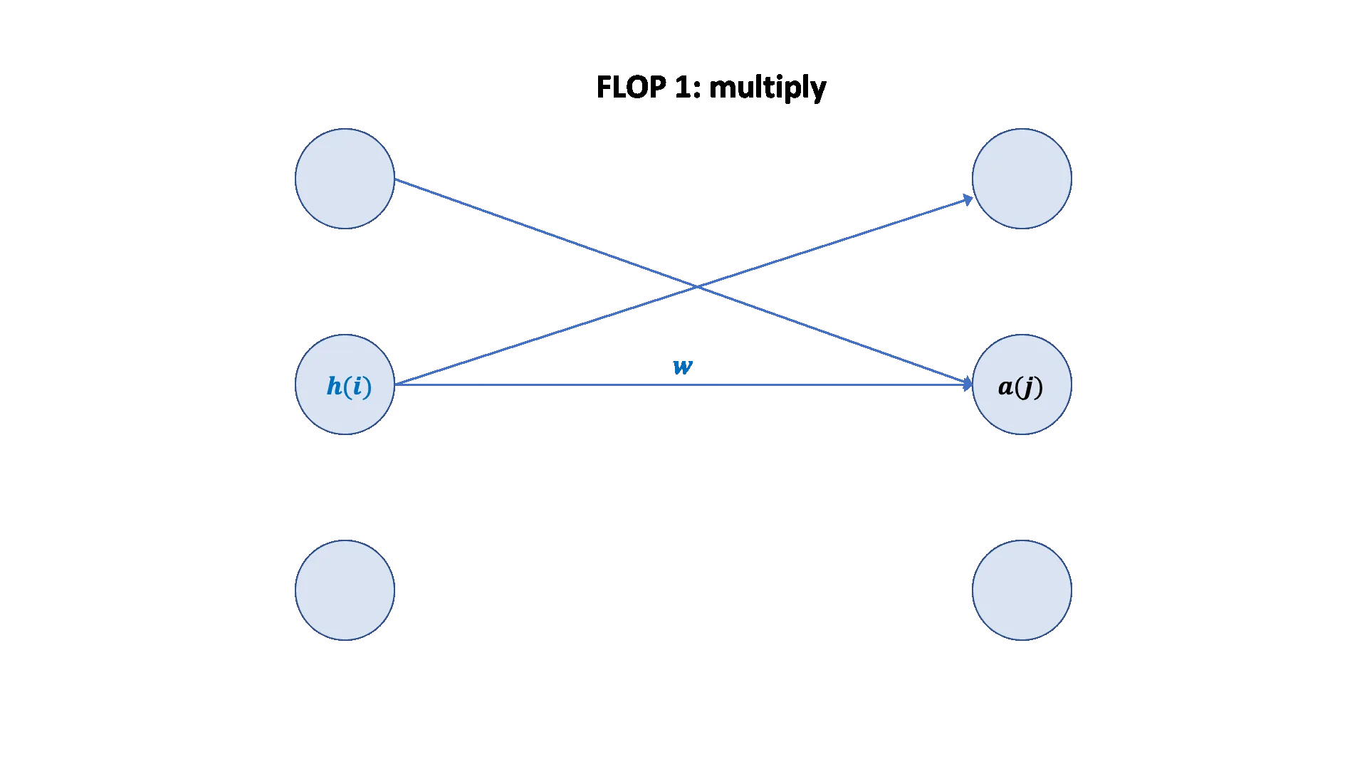
浮点运算数（FLOPs）：
- x @ w 涉及一次乘法和一次加法。
- 每个输出值都需要D次乘法和D−1次加法，共约2D次运算。
- 总的FLOPs为2×B×D×K。

python

import torch

# 根据是否有 GPU 调整矩阵大小
if torch.cuda.is_available():
    B = 16384  # 点的数量 (batch size)
    D = 32768  # 特征维度
    K = 8192   # 输出维度
else:
    B = 1024
    D = 256
    K = 64

# 获取设备 (CPU 或 GPU)
device = torch.device("cuda" if torch.cuda.is_available() else "cpu")

# 输入张量和权重矩阵
x = torch.ones(B, D, device=device)
w = torch.randn(D, K, device=device)

# 矩阵乘法
y = x @ w
print("y.shape:", y.shape)  # torch.Size([B, K])

# =========================================
# 计算 FLOPs (浮点运算量)
# =========================================
# 对每个 (i, j, k) 三元组有一次乘法和一次加法
flops = B * D * K * 2
print(f"FLOPs for this matmul: {flops:.2e}")

其他操作的FLOPs

逐元素操作（Elementwise operation）：对一个m×n矩阵进行逐元素操作，所需的FLOPs约为O(mn)。
矩阵加法：两个m×n矩阵相加，需要mn次浮点运算。
总结：在深度学习中，对于足够大的矩阵，矩阵乘法的计算成本远高于其他操作。

浮点运算与实际时间

理论与实际：线性模型前向传播的FLOPs可以概括为**2×(tokens)×(parameters)，**这一规律在Transformer模型中也大致适用。
计算实际时间：
- actual_time：通过对矩阵乘法进行计时获得实际耗时（以秒为单位）。
- actual_flop_per_sec：用总的FLOPs除以实际耗时，得到每秒的实际浮点运算次数。
python
```
    actual_time = time_matmul(x, w)  # @inspect actual_time
    actual_flop_per_sec = actual_num_flops / actual_time  # @inspect actual_flop_per_sec
```
峰值性能：每个GPU都有一个规格表，会报告其峰值性能（如A100和H100）**[spec] [spec]**。**每秒浮点运算数（FLOP/s）**会根据使用的数据类型（如FP32、FP16）有很大差异。

模型浮点运算利用率（MFU）

定义：MFU是**实际浮点运算速度（actual FLOP/s）与理论峰值浮点运算速度（promised FLOP/s）**的比值。在计算时，可以忽略通信和开销的影响。
计算公式：MFU = actual_flop_per_sec / promised_flop_per_sec
评判标准：通常情况下，MFU达到0.5或更高就算相当不错，如果计算任务主要由矩阵乘法主导，MFU会更高。

BFloat16数据类型示例

将数据类型从float32切换到bfloat16后，实际浮点运算速度（bf16_actual_flop_per_sec）会变高。
然而，示例中的MFU值较低，这可能是因为理论峰值（promised FLOPs）的计算过于乐观。

python

import torch

# =========================================
# 使用 bfloat16 进行矩阵乘法并计算 MFU
# =========================================

# 假设 x, w 已经定义好并在合适的设备上
# x: torch.Tensor of shape [B, D]
# w: torch.Tensor of shape [D, K]

# 转为 bfloat16 以加速计算
x = x.to(torch.bfloat16)
w = w.to(torch.bfloat16)

# 测量实际矩阵乘法时间
bf16_actual_time = time_matmul(x, w)  # @inspect bf16_actual_time
print("Actual time (bf16):", bf16_actual_time)

# 计算实际 FLOPs/s
bf16_actual_flop_per_sec = actual_num_flops / bf16_actual_time  # @inspect bf16_actual_flop_per_sec
print("Actual FLOPs/s (bf16):", bf16_actual_flop_per_sec)

# 获取设备理论峰值 FLOPs/s
bf16_promised_flop_per_sec = get_promised_flop_per_sec(device, x.dtype)  # @inspect bf16_promised_flop_per_sec
print("Promised FLOPs/s (bf16):", bf16_promised_flop_per_sec)

# 计算最大填充利用率 (MFU)
bf16_mfu = bf16_actual_flop_per_sec / bf16_promised_flop_per_sec
print("MFU (bfloat16):", bf16_mfu)

# 说明：
# - bfloat16 可以在保持精度的同时提高吞吐量
# - MFU(Maximum Filling Utilization) 衡量硬件利用效率

总结

矩阵乘法：计算量在深度学习中占主导地位，其浮点运算数（FLOPs）约为2×m×n×p。
FLOP/s：每秒浮点运算数取决于硬件（例如H100优于A100）和数据类型（例如bfloat16的性能通常优于float32）。
模型浮点运算利用率（MFU）：MFU是实际的FLOP/s与理论峰值FLOP/s的比值。

gradients

梯度计算基础

前向传播：将张量（数据或参数）通过一系列操作得到损失（loss）。
反向传播：根据损失计算出每个参数的梯度（gradient），即损失函数对参数的导数。

示例：简单线性模型

模型函数： $y = 0.5 (x * w - 5)^2$
前向传播：
- x：输入张量 [1., 2, 3]。
- w：参数张量 [1., 1, 1]，设置 requires_grad=True 以便计算梯度。
- 预测值 pred_y：x @ w 得到 1*1 + 2*1 + 3*1 = 6。
- 损失 loss：0.5 * (6 - 5)^2 = 0.5。
反向传播：
- loss.backward() 执行反向传播，自动计算梯度。
- 最终，参数 w 的梯度为**[1, 2, 3]*。
- 值得注意的是，loss、pred_y 和 x 等没有设置 requires_grad=True 的张量，其梯度为 None。

python

import torch

# =========================================
# 简单线性模型正向和反向传播
# =========================================

x = torch.tensor([1., 2., 3])
w = torch.tensor([1., 1, 1], requires_grad=True)

# 前向传播
pred_y = x @ w
loss = 0.5 * (pred_y - 5).pow(2)

# 反向传播
loss.backward()

# 检查梯度
assert loss.grad is None
assert pred_y.grad is None
assert x.grad is None
assert torch.equal(w.grad, torch.tensor([1., 2., 3]))

gradient flops

前向传播 FLOPs

对于给定的线性模型：x --w1--> h1 --w2--> h2，其前向传播的总FLOPs等于两次矩阵乘法的FLOPs之和。

x @ w1：矩阵维度为 (B, D) 和 (D, D)。FLOPs为 2 * B * D * D。
h1 @ w2：矩阵维度为 (B, D) 和 (D, K)。FLOPs为 2 * B * D * K。

因此，前向传播总FLOPs = (2 * B * D * D) + (2 * B * D * K)。

反向传播 FLOPs

反向传播（梯度计算）的FLOPs是前向传播的两倍。

计算 w2 的梯度：w2.grad 的计算涉及 h1 和 h2.grad 的矩阵乘法，这与前向传播中 h1 @ w2 的计算量类似。FLOPs约为 2 * B * D * K。
计算 h1 的梯度：h1.grad 的计算涉及 h2.grad 和 w2 的矩阵乘法，FLOPs约为 2 * B * D * K。
计算 w1 和 x 的梯度：这一步的计算量类似。其中，w1.grad 涉及 x 和 h1.grad 的矩阵乘法，FLOPs约为 2 * B * D * D；x.grad 涉及 h1.grad 和 w1 的矩阵乘法，FLOPs约为 2 * B * D * D。

因此，反向传播总FLOPs = (2 * B * D * K) + (2 * B * D * K) + (2 * B * D * D) + (2 * B * D * D)，约等于前向传播总FLOPs的两倍。

前向传播：FLOPs约为**2 * (数据点数) * (参数数量)*。
反向传播：FLOPs约为**4 * (数据点数) * (参数数量)*。
总FLOPs：训练过程的总FLOPs（前向 + 反向）约为**6 * (数据点数) * (参数数量)*。

A nice graphical visualization: [article]

content-image-1

python

import torch

# =========================================
# 计算线性模型的前向和反向 FLOPs
# =========================================

# 设置矩阵大小
if torch.cuda.is_available():
    B, D, K = 16384, 32768, 8192
else:
    B, D, K = 1024, 256, 64

device = torch.device("cuda" if torch.cuda.is_available() else "cpu")

# 定义输入和参数
x = torch.ones(B, D, device=device)
w1 = torch.randn(D, D, device=device, requires_grad=True)
w2 = torch.randn(D, K, device=device, requires_grad=True)

# 前向传播
h1 = x @ w1
h2 = h1 @ w2
loss = h2.pow(2).mean()

# 计算前向 FLOPs
num_forward_flops = (2 * B * D * D) + (2 * B * D * K)  # @inspect num_forward_flops

# 保留中间梯度
h1.retain_grad()
h2.retain_grad()

# 反向传播
loss.backward()

# 计算 w2 相关的反向 FLOPs
num_backward_flops = 0
num_backward_flops += 2 * B * D * K  # w2.grad
num_backward_flops += 2 * B * D * K  # h1.grad
num_backward_flops += (2 + 2) * B * D * D  # w1.grad  # @inspect num_backward_flops

# 检查维度
assert w2.grad.size() == torch.Size([D, K])
assert h1.size() == torch.Size([B, D])
assert h2.grad.size() == torch.Size([B, K])
assert h1.grad.size() == torch.Size([B, D])
assert w2.size() == torch.Size([D, K])

模型参数

存储方式：模型参数在PyTorch中nn.Parameter对象的形式存储，它本质上是一种特殊的张量（torch.Tensor），可以通过 .data 属性访问底层张量。

参数初始化

问题：当未经过特殊初始化时，模型输出的数值会随着输入维度（input_dim）的增加而不成比例地增大，其增长速率为 $\sqrt{\text{input_dim}}$ 。这可能导致梯度爆炸，使模型训练变得不稳定。
解决方案：为了使输出值不受输入维度的影响，需要对参数进行重新缩放，方法是将参数除以1/sqrt(input_dim)。
结果：重新缩放后，模型的输出值将保持在一个恒定的范围内，从而使得训练更稳定。
初始化方法：这种重新缩放的初始化方法，在加入常数因子后，即为Xavier初始化。
额外安全措施：为了避免正态分布中可能出现的离群值（outliers），可以额外将正态分布截断到[-3, 3]的范围内。

python

import torch
import torch.nn as nn
import numpy as np

input_dim, output_dim = 16384, 32

# 模型参数是 nn.Parameter
w = nn.Parameter(torch.randn(input_dim, output_dim))
assert isinstance(w, torch.Tensor)
assert isinstance(w.data, torch.Tensor)

# 普通初始化 -> 输出随 √input_dim 变大
x = nn.Parameter(torch.randn(input_dim))
out1 = x @ w  # ~ O(√input_dim)

# Xavier 初始化 (缩放 1/√input_dim)
w2 = nn.Parameter(torch.randn(input_dim, output_dim) / np.sqrt(input_dim))
out2 = x @ w2  # ~ O(1)

# 截断正态分布 (更安全)
w3 = nn.Parameter(
    nn.init.trunc_normal_(
        torch.empty(input_dim, output_dim),
        std=1 / np.sqrt(input_dim),
        a=-3, b=3
    )
)
out3 = x @ w3  # ~ O(1)

Custom model

python

import torch
import torch.nn as nn
import numpy as np

# ---- 定义简单线性层 ----
class Linear(nn.Module):
    """Simple linear layer."""
    def __init__(self, input_dim: int, output_dim: int):
        super().__init__()
        self.weight = nn.Parameter(
            torch.randn(input_dim, output_dim) / np.sqrt(input_dim)
        )

    def forward(self, x: torch.Tensor) -> torch.Tensor:
        return x @ self.weight

# ---- 定义深度线性模型 ----
class Cruncher(nn.Module):
    def __init__(self, dim: int, num_layers: int):
        super().__init__()
        self.layers = nn.ModuleList([
            Linear(dim, dim) for _ in range(num_layers)
        ])
        self.final = Linear(dim, 1)

    def forward(self, x: torch.Tensor) -> torch.Tensor:
        B, D = x.size()
        for layer in self.layers:
            x = layer(x)
        # Final projection
        x = self.final(x)
        assert x.size() == torch.Size([B, 1])
        return x.squeeze(-1)

# ---- 工具函数 ----
def get_num_parameters(model: nn.Module) -> int:
    return sum(p.numel() for p in model.parameters())

def get_device() -> torch.device:
    return torch.device("cuda" if torch.cuda.is_available() else "cpu")

# ---- custom_model 示例 ----
def custom_model():
    D = 64   # Dimension
    num_layers = 2
    model = Cruncher(dim=D, num_layers=num_layers)

    # 检查参数大小
    param_sizes = [(name, param.numel()) for name, param in model.state_dict().items()]
    assert param_sizes == [
        ("layers.0.weight", D * D),
        ("layers.1.weight", D * D),
        ("final.weight", D),
    ]

    # 参数总数
    num_parameters = get_num_parameters(model)
    assert num_parameters == (D * D) + (D * D) + D

    # 移动到 GPU
    device = get_device()
    model = model.to(device)

    # 运行模型
    B = 8  # Batch size
    x = torch.randn(B, D, dev

get batch

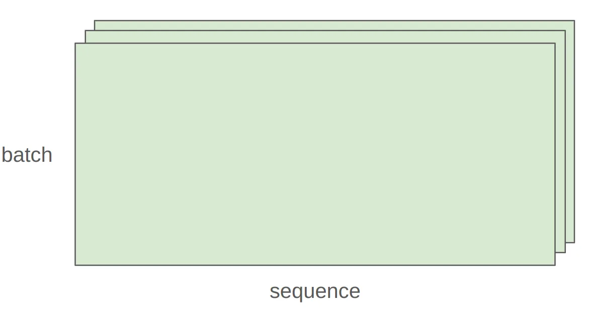
目标：从给定的数据数组 data 中，随机采样出batch_size个序列，每个序列的长度为sequence_length。
实现步骤：
1. 随机采样起始位置：使用 torch.randint 随机生成 batch_size 个起始索引 start_indices，确保每个索引都可以在数据范围内截取一个完整的序列。
2. 索引数据：利用列表推导式，根据 start_indices 索引到 data 中，构建一个大小为 [batch_size, sequence_length] 的输入张量 x。

内存管理与异步传输

固定内存（Pinned Memory）：
- 默认情况下，CPU张量存储在**分页内存（paged memory）**中。
- 通过调用 .pin_memory()，可以将张量显式地放入固定内存中。
异步复制：
- 将张量从固定内存复制到GPU时，可以设置 non_blocking=True。
- 这样做的好处是，CPU可以并行执行其他任务（例如获取下一个数据批次），而无需等待张量复制到GPU完成。
并行优势：这种异步传输机制使得数据加载（在CPU上）和模型计算（在GPU上）可以重叠，从而提高训练效率。

[article]

python

import torch
import numpy as np

def get_batch(data: np.ndarray, batch_size: int, sequence_length: int, device: str) -> torch.Tensor:
    """
    Sample a random batch of sequences from data.
    
    Args:
        data: numpy array of data
        batch_size: number of sequences per batch
        sequence_length: length of each sequence
        device: target device ("cpu" or "cuda")

    Returns:
        x: torch.Tensor [batch_size, sequence_length]
    """
    # 随机选择起始位置
    start_indices = torch.randint(len(data) - sequence_length, (batch_size,))
    assert start_indices.size() == torch.Size([batch_size])

    # 构造 batch
    x = torch.tensor(
        [data[start:start + sequence_length] for start in start_indices],
        dtype=torch.float32
    )
    assert x.size() == torch.Size([batch_size, sequence_length])

    # 固定内存 (提高 CPU→GPU 数据拷贝效率)
    if torch.cuda.is_available():
        x = x.pin_memory()

    # 传输到设备
    x = x.to(device, non_blocking=True)

    return x

随机性与可复现性

随机性来源：随机性出现在多个环节，包括参数初始化、Dropout（一种正则化技术）和数据排序等。
可复现性（Reproducibility）：为了确保每次运行结果一致，尤其在调试时，强烈建议始终为每次随机操作设置一个固定的随机种子（random seed）。
好处：通过固定随机种子，可以确定性地重现模型的行为，从而更容易定位并修复代码中的错误。

设置随机种子

为了确保完全的可复现性，应在三个主要库中同时设置随机种子：

PyTorch：使用 torch.manual_seed(seed)。
NumPy：使用 np.random.seed(seed)。
Python：使用 random.seed(seed)。

数据加载

数据格式：语言模型的数据通常是**分词器（tokenizer）**输出的整数序列。
存储方式：这些序列可以被序列化为numpy数组，并以.npy文件格式存储，以便于加载。

高效加载大型数据集

内存映射（Memory-mapping）：当处理如LLaMA数据集（2.8TB）这样的大型数据集时，不能一次性将所有数据加载到内存中。
np.memmap：numpy的内存映射功能允许**延迟加载（lazily load）**数据。这意味着只有在访问数据文件的特定部分时，才会将其加载到内存中，从而节省了大量的RAM。
数据加载器（data loader）：数据加载器的作用是为训练模型生成一个**批次（batch）**的序列。它会从数据集中采样出固定大小（B）和固定长度（L）的序列，形成一个大小为[B, L]的张量。

SGD（随机梯度下降）

python

class SGD(torch.optim.Optimizer):
    def __init__(self, params: Iterable[nn.Parameter], lr: float = 0.01):
        super(SGD, self).__init__(params, dict(lr=lr))

    def step(self):
        for group in self.param_groups:
            lr = group["lr"]
            for p in group["params"]:
                grad = p.grad.data
                p.data -= lr * grad

特点：

最基础的优化器
更新公式：p = p - lr * grad

AdaGrad

python

class AdaGrad(torch.optim.Optimizer):
    def __init__(self, params: Iterable[nn.Parameter], lr: float = 0.01):
        super(AdaGrad, self).__init__(params, dict(lr=lr))

    def step(self):
        for group in self.param_groups:
            lr = group["lr"]
            for p in group["params"]:
                state = self.state[p]
                grad = p.grad.data
                g2 = state.get("g2", torch.zeros_like(grad))
                g2 += torch.square(grad)
                state["g2"] = g2
                p.data -= lr * grad / torch.sqrt(g2 + 1e-5)

特点：

对梯度平方进行累计
对学习率做自适应缩放

优化器家族关系

Momentum = SGD + 梯度指数平均
AdaGrad = SGD + 梯度平方平均
RMSProp = AdaGrad + 梯度平方指数平均
Adam = RMSProp + Momentum

参考论文：AdaGrad

基本训练流程

python

def train(name: str, get_batch, D: int, num_layers: int, B: int, num_train_steps: int, lr: float):
    model = Cruncher(dim=D, num_layers=num_layers).to(get_device())
    optimizer = SGD(model.parameters(), lr=lr)
    for t in range(num_train_steps):
        x, y = get_batch(B=B)
        pred_y = model(x)
        loss = F.mse_loss(pred_y, y)
        loss.backward()
        optimizer.step()
        optimizer.zero_grad(set_to_none=True)

数据生成示例

python

def get_batch(B: int) -> tuple[torch.Tensor, torch.Tensor]:
    D = 16
    true_w = torch.arange(D, dtype=torch.float32, device=get_device())
    x = torch.randn(B, D).to(get_device())
    true_y = x @ true_w
    return x, true_y

检查点（Checkpointing）

保存训练状态，避免训练中断导致的数据丢失：

python

model = Cruncher(dim=64, num_layers=3).to(get_device())
optimizer = AdaGrad(model.parameters(), lr=0.01)

# 保存
checkpoint = {
    "model": model.state_dict(),
    "optimizer": optimizer.state_dict(),
}
torch.save(checkpoint, "model_checkpoint.pt")

# 加载
loaded_checkpoint = torch.load("model_checkpoint.pt")

混合精度训练（Mixed Precision Training）

高精度（float32）：稳定、准确，但消耗内存和计算
低精度（bfloat16, fp8）：节省资源，但可能不稳定
解决方案：前向传播使用低精度，参数和梯度保持 float32

PyTorch AMP：官方文档

NVIDIA Transformer Engine 支持 FP8：参考论文

内存与 FLOPs 估算

python

def get_memory_usage(x: torch.Tensor):
    return x.numel() * x.element_size()

def get_num_parameters(model: nn.Module) -> int:
    return sum(param.numel() for param in model.parameters())

def get_promised_flop_per_sec(device: str, dtype: torch.dtype) -> float:
    ...

示例：

参数数量：num_parameters = D*D*num_layers + D
激活数量：num_activations = B * D * num_layers
梯度数量：num_gradients = num_parameters
优化器状态：num_optimizer_states = num_parameters
总内存（float32）：total_memory = 4 * (num_parameters + num_activations + num_gradients + num_optimizer_states)
FLOPs（单步）：flops = 6 * B * num_parameters

工具函数

python

def same_storage(x: torch.Tensor, y: torch.Tensor):
    return x.untyped_storage().data_ptr() == y.untyped_storage().data_ptr()

def time_matmul(a: torch.Tensor, b: torch.Tensor) -> float:
    ...

def get_device(index: int = 0) -> torch.device:
    if torch.cuda.is_available():
        return torch.device(f"cuda:{index}")
    else:
        return torch.device("cpu")

7. 总结

优化器：理解不同算法及其适用场景（SGD, AdaGrad, RMSProp, Adam）
训练流程：数据 -> forward -> loss -> backward -> update
内存与计算：关注参数、激活、梯度、优化器状态
混合精度训练：在保持稳定性的同时节省内存和计算